# Created: 20250103

import pyutil as pyu
pyu.get_local_pyinfo()

'conda env: ml312-2024; pyv: 3.12.7 | packaged by Anaconda, Inc. | (main, Oct  4 2024, 13:27:36) [GCC 11.2.0]'

print(pyu.ps2("requests"))

requests==2.32.3

import yfinance as yf
import pandas as pd
import numpy as np
import matplotlib.pyplot as plt

import yfinance as yf
import pandas as pd
import matplotlib.pyplot as plt

# Step 1: Download historical data
symbol = "^GSPC"  # S&P 500 as an example
start = "2020-01-01"
end = "2023-12-31"
data = yf.download(symbol, start=start, end=end)

# Step 2: Calculate OBV
def calculate_obv(data):
    obv = [0]  # Initialize OBV with zero for the first row

    for i in range(1, len(data)):
        # Extract scalar values for the current and previous Close and Volume
        current_close = data['Close'].iloc[i]
        previous_close = data['Close'].iloc[i - 1]
        current_volume = data['Volume'].iloc[i]

        # Calculate OBV based on price movement
        if current_close > previous_close:
            obv.append(obv[-1] + current_volume)
        elif current_close < previous_close:
            obv.append(obv[-1] - current_volume)
        else:
            obv.append(obv[-1])

    # Add OBV to the DataFrame
    data['OBV'] = obv
    return data

# Apply the OBV calculation
data = calculate_obv(data)

# Step 3: Plot OBV
plt.figure(figsize=(14, 7))

# Plot Close Price
plt.subplot(2, 1, 1)
plt.plot(data['Close'], label='Close Price', color='blue')
plt.title(f'{symbol} Close Price')
plt.xlabel('Date')
plt.ylabel('Price')
plt.legend()
plt.grid(True)

# Plot OBV
plt.subplot(2, 1, 2)
plt.plot(data['OBV'], label='On-Balance Volume (OBV)', color='purple')
plt.title('On-Balance Volume (OBV)')
plt.xlabel('Date')
plt.ylabel('OBV')
plt.legend(loc='best')
plt.grid(True)

plt.tight_layout()
plt.show()

[*********************100%***********************]  1 of 1 completed



---------------------------------------------------------------------------

ValueError                                Traceback (most recent call last)

/tmp/ipykernel_1002167/3899796312.py in ?()
     30     data['OBV'] = obv
     31     return data
     32 
     33 # Apply the OBV calculation
---> 34 data = calculate_obv(data)
     35 
     36 # Step 3: Plot OBV
     37 plt.figure(figsize=(14, 7))


/tmp/ipykernel_1002167/3899796312.py in ?(data)
     18         previous_close = data['Close'].iloc[i - 1]
     19         current_volume = data['Volume'].iloc[i]
     20 
     21         # Calculate OBV based on price movement
---> 22         if current_close > previous_close:
     23             obv.append(obv[-1] + current_volume)
     24         elif current_close < previous_close:
     25             obv.append(obv[-1] - current_volume)


~/miniconda3/envs/ml312-2024/lib/python3.12/site-packages/pandas/core/generic.py in ?(self)
   1575     @final
   1576     def __nonzero__(self) -> NoReturn:
-> 1577         raise ValueError(
   1578             f"The truth value of a {type(self).__name__} is ambiguous. "
   1579             "Use a.empty, a.bool(), a.item(), a.any() or a.all()."
   1580         )


ValueError: The truth value of a Series is ambiguous. Use a.empty, a.bool(), a.item(), a.any() or a.all().

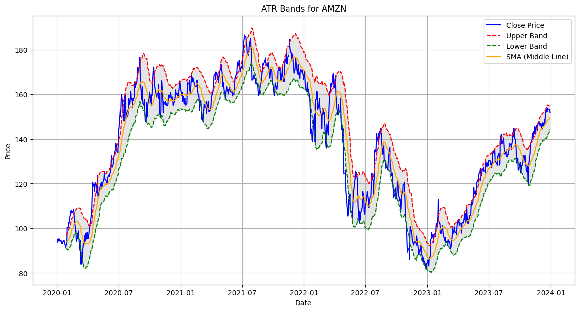
def show_graph(symbol):

pass

show_graph("AMZN")

[*********************100%***********************]  1 of 1 completed