Seaborn-Flight-Data-Analysis
Fri 14 November 2025
# https://seaborn.pydata.org/generated/seaborn.lineplot.html
# https://rajacsp.github.io/mlnotes/python/data-wrangling/food_points/
import seaborn as sns
flights = sns.load_dataset("flights")
flights.head()
| year | month | passengers | |
|---|---|---|---|
| 0 | 1949 | Jan | 112 |
| 1 | 1949 | Feb | 118 |
| 2 | 1949 | Mar | 132 |
| 3 | 1949 | Apr | 129 |
| 4 | 1949 | May | 121 |
type(flights)
pandas.core.frame.DataFrame
may_flights = flights.query("month == 'May'")
sns.lineplot(data=may_flights, x="year", y="passengers")
<Axes: xlabel='year', ylabel='passengers'>

flights.head()
| year | month | passengers | |
|---|---|---|---|
| 0 | 1949 | Jan | 112 |
| 1 | 1949 | Feb | 118 |
| 2 | 1949 | Mar | 132 |
| 3 | 1949 | Apr | 129 |
| 4 | 1949 | May | 121 |
flights_wide = flights.pivot(index="year", columns="month", values="passengers")
flights_wide.head()
| month | Jan | Feb | Mar | Apr | May | Jun | Jul | Aug | Sep | Oct | Nov | Dec |
|---|---|---|---|---|---|---|---|---|---|---|---|---|
| year | ||||||||||||
| 1949 | 112 | 118 | 132 | 129 | 121 | 135 | 148 | 148 | 136 | 119 | 104 | 118 |
| 1950 | 115 | 126 | 141 | 135 | 125 | 149 | 170 | 170 | 158 | 133 | 114 | 140 |
| 1951 | 145 | 150 | 178 | 163 | 172 | 178 | 199 | 199 | 184 | 162 | 146 | 166 |
| 1952 | 171 | 180 | 193 | 181 | 183 | 218 | 230 | 242 | 209 | 191 | 172 | 194 |
| 1953 | 196 | 196 | 236 | 235 | 229 | 243 | 264 | 272 | 237 | 211 | 180 | 201 |
sns.lineplot(data=flights_wide["May"])
<Axes: xlabel='year', ylabel='May'>

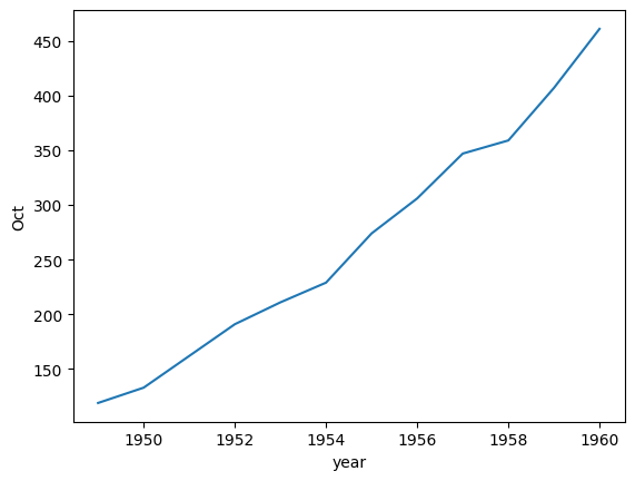
sns.lineplot(data=flights_wide["Oct"])
<Axes: xlabel='year', ylabel='Oct'>
sns.lineplot(data=flights_wide)
<Axes: xlabel='year'>
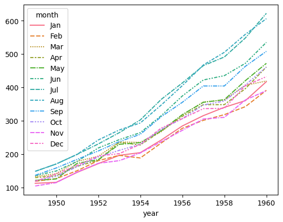
flights_wide
| month | Jan | Feb | Mar | Apr | May | Jun | Jul | Aug | Sep | Oct | Nov | Dec |
|---|---|---|---|---|---|---|---|---|---|---|---|---|
| year | ||||||||||||
| 1949 | 112 | 118 | 132 | 129 | 121 | 135 | 148 | 148 | 136 | 119 | 104 | 118 |
| 1950 | 115 | 126 | 141 | 135 | 125 | 149 | 170 | 170 | 158 | 133 | 114 | 140 |
| 1951 | 145 | 150 | 178 | 163 | 172 | 178 | 199 | 199 | 184 | 162 | 146 | 166 |
| 1952 | 171 | 180 | 193 | 181 | 183 | 218 | 230 | 242 | 209 | 191 | 172 | 194 |
| 1953 | 196 | 196 | 236 | 235 | 229 | 243 | 264 | 272 | 237 | 211 | 180 | 201 |
| 1954 | 204 | 188 | 235 | 227 | 234 | 264 | 302 | 293 | 259 | 229 | 203 | 229 |
| 1955 | 242 | 233 | 267 | 269 | 270 | 315 | 364 | 347 | 312 | 274 | 237 | 278 |
| 1956 | 284 | 277 | 317 | 313 | 318 | 374 | 413 | 405 | 355 | 306 | 271 | 306 |
| 1957 | 315 | 301 | 356 | 348 | 355 | 422 | 465 | 467 | 404 | 347 | 305 | 336 |
| 1958 | 340 | 318 | 362 | 348 | 363 | 435 | 491 | 505 | 404 | 359 | 310 | 337 |
| 1959 | 360 | 342 | 406 | 396 | 420 | 472 | 548 | 559 | 463 | 407 | 362 | 405 |
| 1960 | 417 | 391 | 419 | 461 | 472 | 535 | 622 | 606 | 508 | 461 | 390 | 432 |
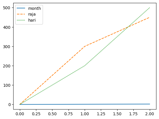
import pandas as pd
data = {
    'month' : [0, 1, 2],
    'raja' : [0, 300, 450],
    'hari' : [0, 200, 500]
}
df = pd.DataFrame(data)
df
| month | raja | hari | |
|---|---|---|---|
| 0 | 0 | 0 | 0 |
| 1 | 1 | 300 | 200 |
| 2 | 2 | 450 | 500 |
sns.lineplot(data=df)
<Axes: >
data = {
    'days' : [1, 1, 1, 2, 2, 2],
    'learners' : ['raja', 'hari', 'steve', 'raja', 'hari', 'steve'],
    'score' : [0, 0, 0, 50, 40, 60]
}

# 1949 Jan 112
# day:1 hari 0
# day:1 steve 0
df = pd.DataFrame(data)
df
| days | learners | score | |
|---|---|---|---|
| 0 | 1 | raja | 0 |
| 1 | 1 | hari | 0 |
| 2 | 1 | steve | 0 |
| 3 | 2 | raja | 50 |
| 4 | 2 | hari | 40 |
| 5 | 2 | steve | 60 |
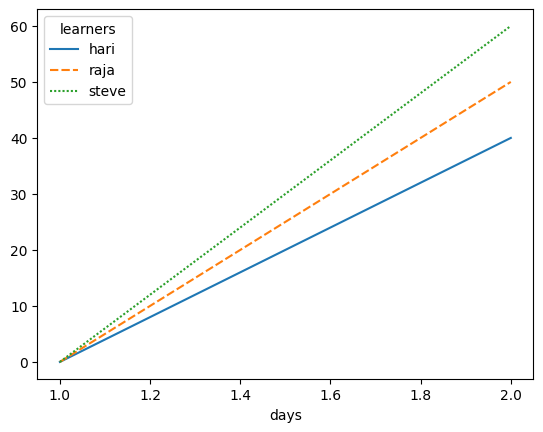
df_wide = df.pivot(index="days", columns="learners", values="score")
df_wide.head()
| learners | hari | raja | steve |
|---|---|---|---|
| days | |||
| 1 | 0 | 0 | 0 |
| 2 | 40 | 50 | 60 |
sns.lineplot(data=df_wide)
<Axes: xlabel='days'>
Score: 20
Category: plot